Order Statistics For the Working Engineer

Imagine you’re writing a program that does one of the following:

• Dispatches a job request to $n$ nodes and assigns the job to the first node to respond
• Writes to $n$ nodes in a cluster and requires $\texttt{ACK}$ from at least three before committing
• Calculates an average of the value of a key across $n$ DB partitions

Dubious claim. Let me give an example. It’s almost certain your system measures percentiles of some primitive operation (e.g. $\texttt{write_to_node}$) and it’s possible your system measures percentiles of some aggregate operation (e.g. $\texttt{quorum_write_nodes}$). This post is about napkin-math’ing timing of aggregate operations using only metrics about the primitive.

These operations depend on the timing of the first, third, and last of $n$ calls respectively. Estimating the timings of operations like these can be challenging when observability systems are built only to measure the performance of single operations. However, if we can assume that response times from $$\texttt{SOME_SERVICE}$ are independent, we can compose an estimate of the timing of the $k^{th}$ of $n$ calls with order statistics.

The order statistics of a random sample are the sample values placed in ascending order. We denote the minimum value from this sample as $X_{\Big(1)}$, the second smallest as $X_{\Big(2)}$, and so forth (i.e. $X_{\Big(1)} \leq X_{\Big(2)} ... \leq X_{\Big(n)}$). Given the CDF ($F_X$) for a single call, the CDF of the $k^{th}$ order statistic of $n$ calls is given as:

$$\begin{equation} F_X_\left(k\right)\Big(x) = \sum_{j=k}^{n} \binom{n}{j} \Big[F_X\big(x)]^j \Big[1 - F_X\big(x)]^{n-j} \end{equation}$$

In some cases we can further simplify an estimate. For example, we can show that the $\textit{minimum}$ of $n$ exponential random variables with parameter $\lambda$ is exponentially distributed with parameter $n\lambda$.

$$\begin{equation} F_X_\left(k\right) \big(x) = 1 - \Big[1 - \big(1 - e^{-\lambda x})]^{n} = 1 - e^{-n\lambda x} \end{equation}$$

In each term of the CDF we calculate the probability that $j$ values are smaller and $n-j$ values are larger than $x$. When using $k = n$ or $k = 1$, we have easier to calculate special cases:

$$\begin{equation} \begin{aligned} F_X_{\Big(n)}\Big(x) & = & Pr\Big(X_{\Big(n)} \leq x) & = & \prod_{k=1}^n Pr\Big(X_k \leq x) & = & {F_{X}\Big(x)}^n \\ F_X_{\Big(1)}\Big(x) & = & Pr\Big(X_{\Big(1)} \leq x) & = & 1 - \prod_{k=1}^n \Big[1 - Pr\Big(X_k \leq x)] & = & 1 - \Big[1 - F_x\Big(x)]^{n} \end{aligned} \end{equation}$$

Reframe our Base CDF. Replace $F_X\colon \mathbb{R} \to \Big(0, 1)$ with $F_X\colon \Big(0, 1) \to \Big(0, 1)$ s.t. $F_X\Big(x) = x, \ x \in \Big(0, 1)$.

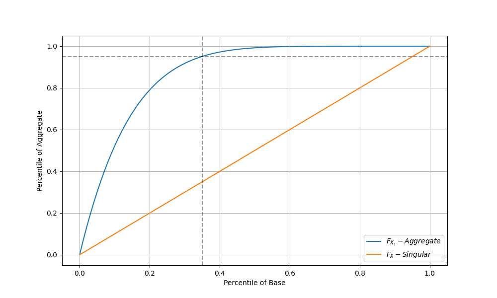
However, we don’t often have closed-form distributions for responses from $$\texttt{SOME_SERVICE}$. Luckily we don’t need them to provide good estimates. Rather than working with a base CDF ($F_X$) that maps response times (in ms) to a percentile (on the unit interval), imagine that our base CDF maps a percentile to itself. Unlike distributions, percentiles of response times are readily available in our observability system.

We can also take the inverse of $F_X_{\Big(k)}$ to make more intuitive statements, e.g. “pXX of the aggregate is pYY of the base”, but we don’t need to belabor this point.

Under this reframing, $F_X_\left(k\right)\Big(p_b) = p_a$ indicates that the $p_b^{th}$ percentile of the singular call maps to the $p_a^{th}$ percentile of the aggregate distribution. Consider an example using the $1^{st}$ response from 7 nodes. The p95 of our aggregate call roughly corresponds to the p35 of the base distribution.

This “trick” is a general property and can be used without involving any parametric distribution of response times. If we wanted to be (slightly) more formal we could take $F^{-1}_X\Big(p_a)$ to get the p95 $\textit{time}$ of this aggregate call, but in most cases a quick glance at the metrics of the base distribution will suffice.